Cross-fault-size Generalization in Bearing Fault Diagnosis: Analysis of Negative Transfer Phenomenon

1. Introduction

Bearings are critical components in rotating machinery across manufacturing, transportation, and energy sectors. Studies indicate that bearing failures account for approximately 40 % ~ 50 % of all rotating machinery failures^(1,2), making early fault detection essential for preventing catastrophic breakdowns and economic losses.

Deep learning, particularly convolutional neural networks (CNNs), has revolutionized bearing fault diagnosis by automatically extracting discriminative features from vibration signals. Recent studies using the Case Western Reserve University (CWRU) benchmark dataset have reported classification accuracies exceeding 99 %⁽³⁾, demonstrating the potential of data-driven approaches. CNN-based methods have been successfully applied to various mechanical systems, achieving high accuracy in classifying multiple fault types from time-frequency representations of sound and vibration signals⁽⁴⁾.

However, a critical gap exists between laboratory performance and real-world reliability. Deep learning models trained under specific conditions often fail to generalize when deployed in environments with different operating parameters. Among various domain shift factors, fault size variation represents a particularly important yet understudied challenge. In real industrial environments, bearing defects progressively grow from microscopic pitting to macroscopic spalling, meaning models trained on specific fault severities must diagnose defects at different progression stages.

This challenge is critical for two practical reasons. First, a minute surface crack with an initial size of approximately 0.1 mm can gradually grow during operation and eventually develop into damage on the order of several millimeters, fundamentally altering the vibration signal characteristics over weeks or months⁽²⁾. This progressive fault growth creates an inherent mismatch between data acquired for model training and data encountered during actual deployment. Second, this problem manifests bidirectionally: models trained on historical data containing primarily large advanced-stage defects may fail to detect subtle incipient faults at deployment, while models trained on precisely machined laboratory defects may struggle to recognize irregular, large defects that develop naturally in operational bearings. Despite this practical significance, most existing studies have treated fault size differences merely as an additional classification dimension (fault severity classification) rather than addressing them as cross-domain generalization challenges.

Furthermore, recent studies have highlighted significant data leakage problems in CWRU benchmark evaluations. Random splitting of time-series data, which allows temporally adjacent segments to appear in both training and test sets, leads to inflated accuracy estimates not reflecting true generalization capability.

The objectives of this research are: (1) to systematically evaluate cross-fault-size generalization through four experimental scenarios (E1-E4); (2) to demonstrate the negative transfer phenomenon where mixing hetero-geneous fault size data degrades performance; (3) to visualize feature space distortion using t-SNE analysis; and (4) to propose practical guidelines for industrial deployment.

2. Theoretical Background

3. Research Methodology

3.3 Experimental Design

Four experiments (E1-E4) were designed to evaluate cross-fault-size generalization. Table 1 summarizes the experimental design.

Table 1

Summary of experimental design (E1-E4) [Unit: mm]

The comparison between E3 and E4 is critical: E3 uses more training data (mixed sizes) while E4 uses validation data from a different fault size domain. This design tests whether data quantity or domain-appropriate validation leads to better generalization.

3.4 Data Preprocessing and CNN Architecture

Raw vibration signals were transformed into STFT spectrograms (see Figure 1) using 64-sample Hann window, 75 % overlap, and 64-point FFT. Spectrograms were converted to decibel scale and resized to 64 × 64 pixels, then normalized to [0, 1] range.

Fig. 1

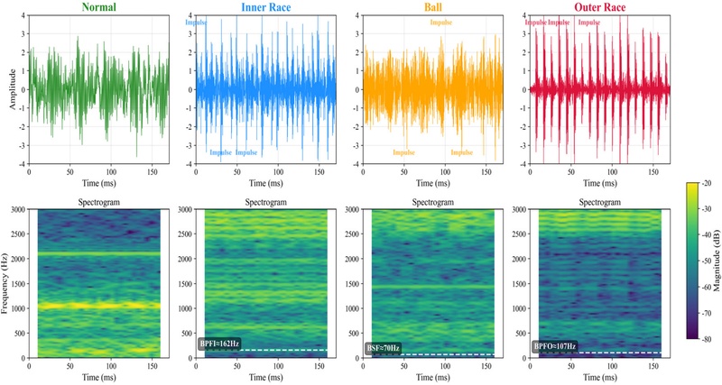
Representative raw vibration signals (top) and full-length STFT spectrograms (bottom) for each fault class, illustrating characteristic frequency patterns. Note: actual CNN inputs are 64 × 64 spectrograms generated from 1024-sample segments using a 64-sample Hann window with 75 % overlap

The CNN architecture consists of three convolutional blocks (32 → 64 → 128 filters) with 3 × 3 kernels, batch normalization, ReLU activation, and 2 × 2 max pooling. Global average pooling followed by a 64-unit dense layer and 4-class softmax output completes the network. Training used Adam optimizer (learning rate 0.001), batch size 16, and early stopping with 7-epoch patience when validation loss showed no improvement. Each experiment was repeated 10 times for statistical reliability.

4. Experimental Results

4.1 Classification Accuracy Analysis

Mean accuracy and standard deviation from 10 repetitions are summarized in Table 2.

Table 2

Mean classification accuracy (10 runs)

E2 achieved the highest mean accuracy (85.3 %), indicating that larger faults produce more distinctive signal patterns that facilitate classification even when trained on smaller faults. The 17.2 percentage point gap between E1 (68.1 %) and E2 (85.3 %) demonstrates significant transfer direction asymmetry.

Most notably, E3 (mixed training, 67.1 %) performed 16.0 percentage points worse than E4 (separated validation, 83.1 %), despite E3 using more diverse training data. Independent samples t-test confirmed this difference is highly statistically significant (t = -6.73, p < 0.001), providing strong evidence of negative transfer (see Figure 2).

Fig. 2

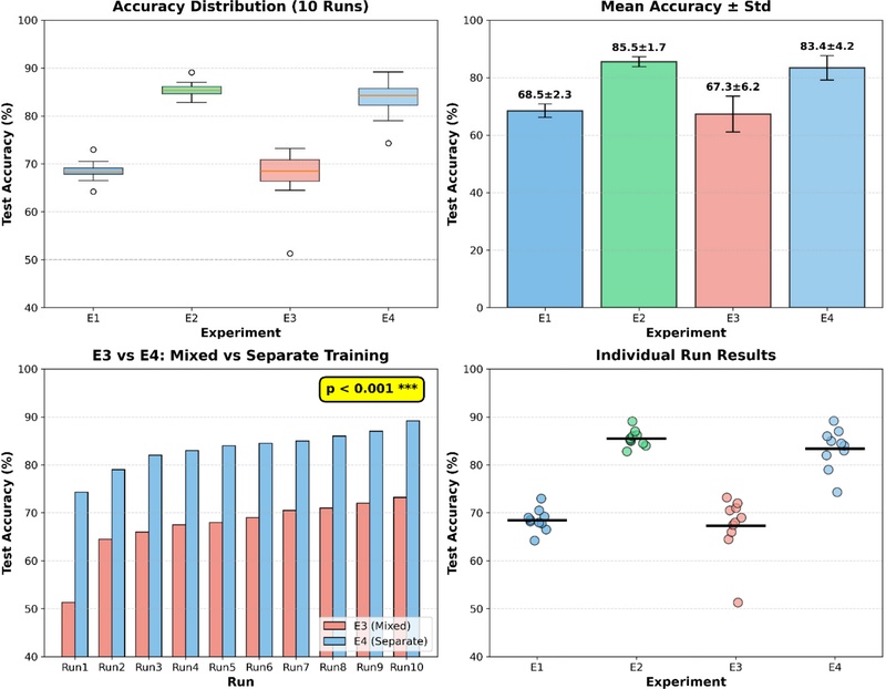
Classification accuracy distribution for each experiment

This counterintuitive result demonstrates that simply combining data from different fault sizes can degrade generalization performance. E4’s superior performance suggests that using validation data from a different domain (0.3556 mm) than training data (0.1778 mm) enables model selection optimized for cross-domain generalization.

4.2 Feature Space Visualization

To understand the underlying causes of performance differences, t-distributed stochastic neighbor embedding (t-SNE) was applied to visualize the learned feature representations⁽¹¹⁾.

Figure 3 presents t-SNE projections for all four experiments (E1-E4). Note that E1 uses 0.3556 mm test data while E2-E4 use 0.5334 mm test data, so direct visual comparison between E1 and the other experiments requires caution due to differing test domains. The following discussion focuses on the E3 vs. E4 comparison, which share the same 0.5334 mm test domain. The E3 feature space exhibits overlap between inner race and ball clusters, with outer race samples intruding into other class regions, while E4 shows relatively clearer cluster separation.

Fig. 3

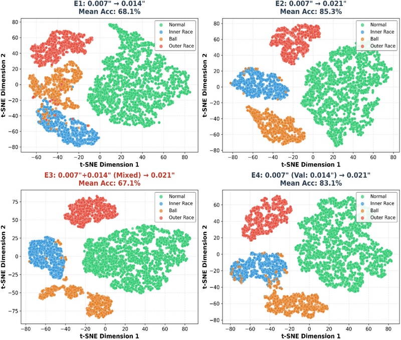
t-SNE feature space visualization (E1-E4). E1 test domain: 0.1778 mm; E2-E4 test domain: 0.5334 mm

However, t-SNE preserves local neighborhood structure but does not faithfully reflect global distance relationships in high-dimensional space, making it difficult to determine whether observed class overlap reflects actual feature distribution distortion or visualization artifacts from dimensionality reduction. Therefore, the following class-wise accuracy comparison (Table 3) and confusion matrix analysis provide independent quantitative verification of t-SNE observations.

Table 3

Class-wise accuracy comparison: E3 vs E4 (mean over 10 runs)

As shown in Table 3, E4 consistently improved performance across all fault classes, with particularly dramatic improvements for inner race (+26.4 %p, from 47.0 % to 73.4 %), ball (+22.6 %p, from 53.1 % to 75.7 %), and outer race (+27.1 %p, from 52.9 % to 80.0 %). These rotating component faults exhibit complex amplitude modulation characteristics that change significantly with fault size, explaining their severe degradation under mixed training. Furthermore, confusion matrix analysis revealed that 21 % of outer race samples were misclassified as inner race in E3, while this rate decreased to 7 % in E4. This misclassification pattern arises because both faults generate similar spectral signatures from impact vibrations as rolling elements pass over the defect; when defect sizes were mixed, the model failed to distinguish these patterns, resulting in decision boundary overlap. These quantitative results independently confirm that the feature space distortion observed in t-SNE reflects actual classification degradation rather than visualization artifacts.

Despite using only 0.1778 mm training data, the E4 model—selected through cross-domain validation using 0.3556 mm data—learned more generalizable features. This suggests that which domain the validation data represents may be more decisive for generalization performance than the quantity of training data itself.

5. Discussion

The experimental results provide clear evidence of negative transfer in fault-size heterogeneous environments^(12,13). E3’s worse performance and higher variance compared to E4 indicates that data from different fault sizes may generate conflicting feature distributions that interfere with learning.

Several mechanisms may explain this negative transfer. First, fault size influences spectral distribution of vibration signals—larger defects generate broader frequency impacts and higher amplitudes. When the model learns from mixed-size data, it may develop averaged feature representations that are suboptimal for any specific size. Second, the optimal decision boundaries for different fault sizes may conflict, causing the model to compromise between incompatible classification criteria.

Transfer direction asymmetry is also noteworthy. The result that E1 (small-to-medium, 68.1 %) performed worse than E2 (small-to-large, 85.3 %) may appear counter-intuitive, as one might expect smaller fault size differences to yield easier transfer. However, this can be explained by bearing vibration dynamics. First, from the signal-to-noise ratio (SNR) perspective, 0.5334 mm large faults produce more pronounced characteristic frequency amplification patterns (BPFO, BPFI, BSF) than 0.3556 mm medium faults, making them easier for models trained on small faults to recognize. Second, small faults generate narrowband energy concentrated around specific characteristic frequencies, while large faults distribute energy across broader frequency bands due to increased contact mechanics nonlinearity. The 0.3556 mm medium fault occupies an intermediate spectral position with high similarity to small fault patterns, making it difficult to distinguish, whereas 0.5334 mm large faults produce qualitatively different spectral patterns that are paradoxically easier to classify. Third, larger defects allow rolling elements to generate multiple impacts per revolution as they enter and exit the damage zone, providing richer diagnostic information in the spectrum. In summary, transfer performance is governed not by the absolute magnitude of fault size difference, but by the qualitative distinctiveness of spectral signatures^(2,5).

These findings have important consequences for AI-based fault diagnosis systems in industrial environments⁽¹⁴⁾. In real predictive maintenance scenarios, the distribution of fault progression stages differs between training and deployment—models trained on specific fault severities must diagnose defects at various stages of degradation.

Based on our findings, the following strategies are suggested: (1) validation data domain design: validation data should represent deployment scenarios rather than matching training data distribution. (2) caution with mixed data: rather than simply combining data from different fault sizes, consider domain-specific learning approaches. (3) performance gap awareness: models achieving over 99 % accuracy in training may perform significantly worse in actual deployment.

6. Conclusion

This study investigated cross-fault-size generalization in deep learning-based bearing fault diagnosis and demonstrated the negative transfer phenomenon through systematic experiments.

The main findings are summarized as follows. First, larger fault sizes produced more distinctive signal patterns, with E2 (small → large transfer) achieving the highest accuracy of 85.3 %.

Second, mixed training (E3) performed 16.0 percentage points worse than separated validation (E4), demonstrating statistically significant negative transfer (p < 0.001). This challenges the assumption that more diverse training data always improves generalization.

Third, t-SNE visualization supplemented by class-wise accuracy analysis and confusion matrix patterns confirmed that mixed training causes feature space distortion where originally separable fault classes become entangled. In particular, outer race to inner race misclassification decreased from 21 % (E3) to 7 % (E4), providing quantitative evidence that separated validation maintains clearer class boundaries.

Fourth, validation data domain selection proved more important than training data quantity for cross-domain generalization.

These findings provide practical guidelines for developing robust bearing diagnosis systems in industrial environments where fault sizes inevitably vary during equipment lifecycle. Future research should explore domain adaptation methods specialized for fault size variation and curriculum learning strategies⁽¹⁵⁾. Additionally, systematic feature space analysis using PCA-based visualization and quantitative clustering metrics such as Silhouette score and Davies-Bouldin index would provide more rigorous characterization of feature distribution changes across different training configurations.

References

• Lei, Y., Yang, B., Jiang, X., Jia, F., Li, N. et al., 2020, Applications of Machine Learning to Machine Fault Diagnosis: A Review and Roadmap, Mechanical Systems and Signal Processing, Vol. 138, 106587. [https://doi.org/10.1016/j.ymssp.2019.106587]
• Randall, R. B. and Antoni, J., 2011, Rolling Element Bearing Diagnostics—A Tutorial, Mechanical Systems and Signal Processing, Vol. 25, No. 2, pp. 485~520. [https://doi.org/10.1016/j.ymssp.2010.07.017]
• Loparo, K., 2012, Bearing Vibration Data Set, Case School of Engineering, Case Western Reserve University Bearing Data Center, OH, United States.
• Kim, S. W., An, K., Back, J., Lee, S. K., Lee, C. et al., 2021, Health Monitoring of Power Driving System Using Sound Signal based on Deep Learning, Transactions of the Korean Society for Noise and Vibration Engineering, Vol. 31, No. 1, pp. 47~56. [https://doi.org/10.5050/KSNVE.2021.31.1.047]
• Antoni, J., 2006, The Spectral Kurtosis: A Useful Tool for Characterising Non-stationary Signals, Mechanical Systems and Signal Processing, Vol. 20, No. 2, pp. 282~307. [https://doi.org/10.1016/j.ymssp.2004.09.001]
• Le Cun, Y., Bengio, Y. and Hinton, G., 2015, Deep Learning, Nature, Vol. 521, No. 7553, pp. 436~444. [https://doi.org/10.1038/nature14539]
• Zhang, W., Li, C., Peng, G., Chen, Y. and Zhang, Z., 2018, A Deep Convolutional Neural Network with New Training Methods for Bearing Fault Diagnosis under Noisy Environment and Different Working Load, Mechanical Systems and Signal Processing, Vol. 100, pp. 439~453. [https://doi.org/10.1016/j.ymssp.2017.06.022]
• Hendriks, J., Dumond, P. and Knox, D. A., 2022, Towards Better Benchmarking using the CWRU Bearing Fault Dataset, Mechanical Systems and Signal Processing, Vol. 169, 108732. [https://doi.org/10.1016/j.ymssp.2021.108732]
• Smith, W. A. and Randall, R. B., 2015, Rolling Element Bearing Diagnostics Using the Case Western Reserve University Data: A Benchmark Study, Mechanical Systems and Signal Processing, Vol. 64~65, pp. 100~131. [https://doi.org/10.1016/j.ymssp.2015.04.021]
• Rauber, T. W., Silva Loca, A. L., Boldt, F., Rodrigues, A. L. and Varejão, F. M., 2021, An Experimental Methodology to Evaluate Machine Learning Methods for Fault Diagnosis, Expert Systems with Applications, Vol. 165, 113953. [https://doi.org/10.1016/j.eswa.2020.114022]
• Maaten, L. and Hinton, G., 2008, Visualizing High-dimensional Data Using t-SNE, Journal of Machine Learning Research, Vol. 9, pp. 2579~2605.
• Pan, S. J. and Yang, Q., 2010, A Survey on Transfer Learning, IEEE Transactions on Knowledge and Data Engineering, Vol. 22, No. 10, pp. 1345~1359. [https://doi.org/10.1109/TKDE.2009.191]
• Zhang, W., Deng, L., Zhang, L. and Wu, D., 2022, A Survey on Negative Transfer, IEEE/CAA Journal of Automatica Sinica, pp. 1~25.
• Du, Y., Wang, A., Wang, S., He, B. and Meng, G., 2020, Fault Diagnosis under Variable Working Conditions Based on STFT and Transfer Deep Residual Network, Shock and Vibration, Vol. 2020, pp. 1~18. [https://doi.org/10.1155/2020/1274380]
• Li, X., Zhang, W., Ding, Q. and Sun, J. Q., 2019, Multi-layer Domain Adaptation Method for Rolling Bearing Fault Diagnosis, Signal Processing, Vol. 157, pp. 180~197. [https://doi.org/10.1016/j.sigpro.2018.12.005]